Pairwise comparison

The residue by residue scores $W_{ij}$ can be used directly in the sequence alignment algorithm of Needleman & Wunsch [Needleman & Wunsch, 1970] to obtain the comparison of two protein sequences or structures. The only difference between the two types of comparison is in the type of the comparison matrix. In the case of sequence, the amino acid substitution matrix is used. In the case of 3D structure, the Euclidean distance (or some function of it) between two equivalent atoms in the current optimal superposition is used [Šali & Blundell, 1990].

The problem of the optimal alignment of two sequences as addressed by the algorithm of Needleman & Wunsch is as follows. We are given two sequences of elements and an $M$ times $N$ score matrix $\cal W$ where $M$ and $N$ are the numbers of elements in the first and second sequence. The scoring matrix is composed of scores $W_{ij}$ describing differences between elements $i$ and $j$ from the first and second sequence respectively. The goal is to obtain an optimal set of equivalences that match elements of the first sequence to the elements of the second sequence. The equivalence assignments are subject to the following “progression rule”: for elements $i$ and $k$ from the first sequence and elements $j$ and $l$ from the second sequence, if element $i$ is equivalenced to element $j$, if element $k$ is equivalenced to element $l$ and if $k$ is greater than $i$, $l$ must also be greater than $j$. The optimal set of equivalences is the one with the smallest alignment score. The alignment score is a sum of scores corresponding to matched elements, also increased for occurrences of non-equivalenced elements (ie gaps). For a detailed discussion of this and related problems see [Sankoff & Kruskal, 1983].

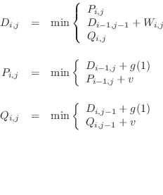
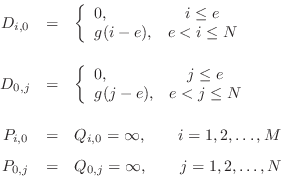
We summarize the dynamic programming formulae used by MODELLER to obtain the optimal alignment since they differ slightly from those already published [Sellers, 1974,Gotoh, 1982]. The recursive dynamic programming formulae that give a matrix $\cal D$ are:

$$\begin{array}{ccl} D_{i,j} & = & \min \left\{ \begin{array}{l... ...\ Q_{i,j-1} + v \end{array} \right. \vspace{0.7in} \end{array}$$ (A.1)

where $g(l)$ is a linear gap penalty function:

$$g(l) = u + v \cdot l \, .$$ (A.2)

Note that only a vector is needed for the storage of $P$ and $Q$. The uppermost formula in Eq. A.1 is calculated for $i=M$ and $j=N$. Variable $l$ is a gap length and parameters $u$ and $v$ are gap-penalty constants.

The arrays $\cal D$, $\cal P$ and $\cal Q$ are initialized as follows:

$$\begin{array}{ccl} D_{i,0} & = & \left\{ \begin{array}{lc} 0,... ...j} & = & Q_{0,j} = \infty , \qquad j = 1,2,\ldots,N \end{array}$$ (A.3)

where parameter $e$ is the maximal number of elements at sequence termini which are not penalized with a gap-penalty if not equivalenced. A segment at the terminus of length $e$ is termed an “overhang”. Note a difference from [Gotoh, 1982] in the initialization of the $\cal P$ and $\cal Q$ arrays. Also note that only vectors $Q_i$ and $P_j$ need to be stored in computer, not the whole arrays.

The minimal score $d_{M,N}$ is obtained from

$$d_{M,N} = \min(D_{i,N}, D_{M,j})$$ (A.4)

where $i = M,M-1,\ldots,M-e \quad \hbox{and} \quad j = N,N-1,\ldots,N-e$ to allow for the overhangs. The equivalence assignments are obtained by backtracking in matrix $\cal D$. Backtracking starts from the element $D_{i,j} = d_{M,N}$.