

Tutorial
Basic example:
Modeling lactate dehydrogenase from Trichomonas vaginalis based on a
single template.
All input and output files for this example are available to download, in either zip format (for Windows) or .tar.gz format (for Unix/Linux).
A novel gene for lactate dehydrogenase was identified from the genomic sequence of Trichomonas vaginalis (TvLDH). The corresponding protein had a higher similarity to the malate dehydrogenase of the same species (TvMDH) than to any other LDH. We hypothesized that TvLDH arose from TvMDH by convergent evolution relatively recently. Comparative models were constructed for TvLDH and TvMDH to study the sequences in the structural context and to suggest site-directed mutagenesis experiments for elucidating specificity changes in this apparent case of convergent evolution of enzymatic specificity. The native and mutated enzymes were expressed and their activities were compared.
The individual modeling steps of this example are explained below. Note that we go through every step in this tutorial to build a model knowing only the amino acid sequence. In practice you may already know the related structures, and may even have an alignment from another program, so you can skip one or more steps. Alternatively, for very simple applications you may be able to use the ModWeb web server rather than Modeller itself.
1. Searching for structures related to TvLDH
First, it is necessary to put the target TvLDH sequence into the PIR format readable by MODELLER (file "TvLDH.ali").
>P1;TvLDH
sequence:TvLDH:::::::0.00: 0.00
MSEAAHVLITGAAGQIGYILSHWIASGELYGDRQVYLHLLDIPPAMNRLTALTMELEDCAFPHLAGFVATTDPKA
AFKDIDCAFLVASMPLKPGQVRADLISSNSVIFKNTGEYLSKWAKPSVKVLVIGNPDNTNCEIAMLHAKNLKPEN
FSSLSMLDQNRAYYEVASKLGVDVKDVHDIIVWGNHGESMVADLTQATFTKEGKTQKVVDVLDHDYVFDTFFKKI
GHRAWDILEHRGFTSAASPTKAAIQHMKAWLFGTAPGEVLSMGIPVPEGNPYGIKPGVVFSFPCNVDKEGKIHVV
EGFKVNDWLREKLDFTEKDLFHEKEIALNHLAQGG*
File: TvLDH.ali
The first line contains the sequence code, in the format ">P1;code". The second line with ten fields separated by colons generally contains information about the structure file, if applicable. Only two of these fields are used for sequences, "sequence" (indicating that the file contains a sequence without known structure) and "TvLDH" (the model file name). The rest of the file contains the sequence of TvLDH, with "*" marking its end. The standard one-letter amino acid codes are used. (Note that they must be upper case; some lower case letters are used for non-standard residues. See the file modlib/restyp.lib in the Modeller distribution for more information.)
A search for potentially related sequences of known structure can be performed by the Profile.build() command of MODELLER. The following script, taken line by line, does the following (see file "build_profile.py"):
- Initializes the 'environment' for this modeling run, by creating a new 'Environ' object. Almost all MODELLER scripts require this step, as the new object (which we call here 'env', but you can call it anything you like) is needed to build most other useful objects.
- Creates a new 'SequenceDB' object, calling it 'sdb'. 'SequenceDB' objects are used to contain large databases of protein sequences.
- Reads a text format file containing non-redundant PDB sequences at 95% sequence identity into the sdb database. The sequences can be found in the file "pdb_95.pir" (which can be downloaded using the link at the top of this page). Like the previously-created alignment, this file is in PIR format. Sequences which have fewer than 30 or more than 4000 residues are discarded, and non-standard residues are removed.
- Writes a binary machine-specific file containing all sequences read in the previous step.
- Reads the binary format file back in. Note that if you plan to use the same database several times, you should use the previous two steps only the first time, to produce the binary database. On subsequent runs, you can omit those two steps and use the binary file directly, since reading the binary file is a lot faster than reading the PIR file.
- Creates a new 'Alignment' object, calling it 'aln', reads our query sequence "TvLDH" from the file "TvLDH.ali", and converts it to a profile 'prf'. Profiles contain similar information to alignments, but are more compact and better for sequence database searching.
- Searches the sequence database 'sdb' for our query profile 'prf'. Matches from the sequence database are added to the profile.
- Writes a profile of the query sequence and its homologs (see file "build_profile.prf"). The equivalent information is also written out in standard alignment format.
from modeller import *

log.verbose()
env = Environ()

#-- Prepare the input files

#-- Read in the sequence database
sdb = SequenceDB(env)
sdb.read(seq_database_file='pdb_95.pir', seq_database_format='PIR',
         chains_list='ALL', minmax_db_seq_len=(30, 4000), clean_sequences=True)

#-- Write the sequence database in binary form
sdb.write(seq_database_file='pdb_95.bin', seq_database_format='BINARY',
          chains_list='ALL')

#-- Now, read in the binary database
sdb.read(seq_database_file='pdb_95.bin', seq_database_format='BINARY',
         chains_list='ALL')

#-- Read in the target sequence/alignment
aln = Alignment(env)
aln.append(file='TvLDH.ali', alignment_format='PIR', align_codes='ALL')

#-- Convert the input sequence/alignment into
#   profile format
prf = aln.to_profile()

#-- Scan sequence database to pick up homologous sequences
prf.build(sdb, matrix_offset=-450, rr_file='${LIB}/blosum62.sim.mat',
          gap_penalties_1d=(-500, -50), n_prof_iterations=1,
          check_profile=False, max_aln_evalue=0.01)

#-- Write out the profile in text format
prf.write(file='build_profile.prf', profile_format='TEXT')

#-- Convert the profile back to alignment format
aln = prf.to_alignment()

#-- Write out the alignment file
aln.write(file='build_profile.ali', alignment_format='PIR')
File: build_profile.py
This is a regular Python script, and so can be run with a command similar to the following at your command line:
python3 build_profile.py > build_profile.log
Note that on some systems the Python interpreter is called python2 or python rather than python3. The full path to the Python interpreter may also be necessary, such as /usr/bin/python on a Linux or Mac machine or C:\python27\python.exe on a Windows system. If Python is not installed on your machine, Modeller also includes a basic Python 2.3 interpeter as mod<version>. For example, to run this script using Modeller 10.0's own interpreter, use mod10.0 build_profile.py. Note that mod10.0 automatically creates a build_profile.log logfile.
(You can get a command line using xterm or GNOME Terminal in Linux, Terminal in Mac OS X, or the 'Modeller' link from your Start Menu in Windows. For more information on running Modeller, see the release notes. For more information on using Python, see the Python web site. Note that you can use other Python modules within your Modeller scripts, if Python is correctly installed on your system.)
The Profile.build() command has many options. In this example rr_file is set to use the BLOSUM62 similarity matrix (file "blosum62.sim.mat" provided in the MODELLER distribution). Accordingly, the parameters matrix_offset and gap_penalties_1d are set to the appropriate values for the BLOSUM62 matrix. For this example, we will run only one search iteration by setting the parameter n_prof_iterations equal to 1. Thus, there is no need for checking the profile for deviation (check_profile set to False). Finally, the parameter max_aln_evalue is set to 0.01, indicating that only sequences with e-values smaller than or equal to 0.01 will be included in the final profile.
2. Selecting a template
The output of the "build_profile.py" script is written to the "build_profile.log" file. MODELLER always produces a log file. Errors and warnings in log files can be found by searching for the "_E>" and "_W>" strings, respectively. MODELLER also writes the profile in text format to the "build_profile.prf" file. An extract (omitting the aligned sequences) of the output file can be seen next. The first 6 commented lines indicate the input parameters used in MODELLER to build the profile. Subsequent lines correspond to the detected similarities by Profile.build().
# Number of sequences:     30
# Length of profile  :    335
# N_PROF_ITERATIONS  :      1
# GAP_PENALTIES_1D   :   -900.0   -50.0
# MATRIX_OFFSET      :    0.0
# RR_FILE            : ${MODINSTALL8v1}/modlib//as1.sim.mat
    1 TvLDH                                    S     0   335     1   335     0     0     0    0.    0.0
    2 1a5z                                     X     1   312    75   242    63   229   164   28.   0.83E-08
    3 1b8pA                                    X     1   327     7   331     6   325   316   42.    0.0
    4 1bdmA                                    X     1   318     1   325     1   310   309   45.    0.0
    5 1t2dA                                    X     1   315     5   256     4   250   238   25.   0.66E-04
    6 1civA                                    X     1   374     6   334    33   358   325   35.    0.0
    7 2cmd                                     X     1   312     7   320     3   303   289   27.   0.16E-05
    8 1o6zA                                    X     1   303     7   320     3   287   278   26.   0.27E-05
    9 1ur5A                                    X     1   299    13   191     9   171   158   31.   0.25E-02
   10 1guzA                                    X     1   305    13   301     8   280   265   25.   0.28E-08
   11 1gv0A                                    X     1   301    13   323     8   289   274   26.   0.28E-04
   12 1hyeA                                    X     1   307     7   191     3   183   173   29.   0.14E-07
   13 1i0zA                                    X     1   332    85   300    94   304   207   25.   0.66E-05
   14 1i10A                                    X     1   331    85   295    93   298   196   26.   0.86E-05
   15 1ldnA                                    X     1   316    78   298    73   301   214   26.   0.19E-03
   16 6ldh                                     X     1   329    47   301    56   302   244   23.   0.17E-02
   17 2ldx                                     X     1   331    66   306    67   306   227   26.   0.25E-04
   18 5ldh                                     X     1   333    85   300    94   304   207   26.   0.30E-05
   19 9ldtA                                    X     1   331    85   301    93   304   207   26.   0.10E-05
   20 1llc                                     X     1   321    64   239    53   234   164   26.   0.20E-03
   21 1lldA                                    X     1   313    13   242     9   233   216   31.   0.31E-07
   22 5mdhA                                    X     1   333     2   332     1   331   328   44.    0.0
   23 7mdhA                                    X     1   351     6   334    14   339   325   34.    0.0
   24 1mldA                                    X     1   313     5   198     1   189   183   26.   0.13E-05
   25 1oc4A                                    X     1   315     5   191     4   186   174   28.   0.18E-04
   26 1ojuA                                    X     1   294    78   320    68   285   218   28.   0.43E-05
   27 1pzgA                                    X     1   327    74   191    71   190   114   30.   0.16E-06
   28 1smkA                                    X     1   313     7   202     4   198   188   34.    0.0
   29 1sovA                                    X     1   316    81   256    76   248   160   27.   0.93E-03
   30 1y6jA                                    X     1   289    77   191    58   167   109   33.   0.32E-05
File: build_profile.prf
The most important columns in the Profile.build() output are the second, tenth, eleventh and twelfth columns. The second column reports the code of the PDB sequence that was compared with the target sequence. The PDB code in each line is the representative of a group of PDB sequences that share 95% or more sequence identity to each other and have less than 30 residues or 30% sequence length difference. The eleventh column reports the percentage sequence identities between TvLDH and a PDB sequence normalized by the lengths of the alignment (indicated in the tenth column). In general, a sequence identity value above approximately 25% indicates a potential template unless the alignment is short (i.e., less than 100 residues). A better measure of the significance of the alignment is given in the twelfth column by the e-value of the alignment. In this example, six PDB sequences show very significant similarities to the query sequence with e-values equal to 0. As expected, all the hits correspond to malate dehydrogenases (1bdm:A, 5mdh:A, 1b8p:A, 1civ:A, 7mdh:A, and 1smk:A). To select the most appropriate template for our query sequence over the six similar structures, we will use the Alignment.compare_structures() command to assess the structural and sequence similarity between the possible templates (file "compare.py").
from modeller import *

env = Environ()
aln = Alignment(env)
for (pdb, chain) in (('1b8p', 'A'), ('1bdm', 'A'), ('1civ', 'A'),
                     ('5mdh', 'A'), ('7mdh', 'A'), ('1smk', 'A')):
    m = Model(env, file=pdb, model_segment=('FIRST:'+chain, 'LAST:'+chain))
    aln.append_model(m, atom_files=pdb, align_codes=pdb+chain)
aln.malign()
aln.malign3d()
aln.compare_structures()
aln.id_table(matrix_file='family.mat')
env.dendrogram(matrix_file='family.mat', cluster_cut=-1.0)
File: compare.py
In this case, we create an (initially empty) alignment object 'aln' and then use a Python 'for' loop to instruct MODELLER to read each of the PDB files. (Note that in order for this to work, you must have all of the PDB files in the same directory as this script, either downloaded from the PDB website or from the archive linked at the top of this page.) We use the model_segment argument to ask only for a single chain to be read from each PDB file (by default, all chains are read from the file). As each structure is read in, we use the append_model method to add the structure to the alignment.
At the end of the loop, all of the structures are in the alignment, but they are not ideally aligned to each other (append_model creates a simple 1:1 alignment with no gaps). Therefore, we improve this alignment by using malign to calculate a multiple sequence alignment. The malign3d command then performs an iterative least-squares superposition of the six 3D structures, using the multiple sequence alignment as its starting point. The compare_structures command compares the structures according to the alignment constructed by malign3d. It does not make an alignment, but it calculates the RMS and DRMS deviations between atomic positions and distances, differences between the mainchain and sidechain dihedral angles, percentage sequence identities, and several other measures. Finally, the id_table command writes a file with pairwise sequence distances that can be used directly as the input to the dendrogram command (or the clustering programs in the PHYLIP package). dendrogram calculates a clustering tree from the input matrix of pairwise distances, which helps visualizing differences among the template candidates. Excerpts from the log file are shown below (file "compare.log").
Sequence identity comparison (ID_TABLE):

   Diagonal       ... number of residues;
   Upper triangle ... number of identical residues;
   Lower triangle ... % sequence identity, id/min(length).

         1b8pA @11bdmA @11civA @25mdhA @27mdhA @21smkA @2
1b8pA @1      327     194     147     151     153      49
1bdmA @1       61     318     152     167     155      56
1civA @2       45      48     374     139     304      53
5mdhA @2       46      53      42     333     139      57
7mdhA @2       47      49      87      42     351      48
1smkA @2       16      18      17      18      15     313


Weighted pair-group average clustering based on a distance matrix:


                                           .----------------------- 1b8pA @1.9    39.0000
                                           |
                                  .-------------------------------- 1bdmA @1.8    50.5000
                                  |
                              .------------------------------------ 5mdhA @2.4    55.3750
                              |
                              |                                .--- 1civA @2.8    13.0000
                              |                                |
        .---------------------------------------------------------- 7mdhA @2.4    83.2500
        |
      .------------------------------------------------------------ 1smkA @2.5

      +----+----+----+----+----+----+----+----+----+----+----+----+
    86.0600   73.4150   60.7700   48.1250   35.4800   22.8350   10.1900
         79.7375   67.0925   54.4475   41.8025   29.1575   16.5125
Excerpts of the file compare.log
The comparison above shows that 1civ:A and 7mdh:A are almost identical, both sequentially and structurally. However, 7mdh:A has a better crystallographic resolution (2.4Å versus 2.8Å), eliminating 1civ:A. A second group of structures (5mdh:A, 1bdm:A, and 1b8p:A) share some similarities. From this group, 5mdh:A has the poorest resolution leaving for consideration only 1bdm:A and 1b8p:A. 1smk:A is the most diverse structure of the whole set of possible templates. However, it is the one with the lowest sequence identity (34%) to the query sequence. We finally pick 1bdm:A over 1b8p:A and 7mdh:A because of its better crystallographic R-factor (16.9%) and higher overall sequence identity to the query sequence (45%).
3. Aligning TvLDF with the template
A good way of aligning the sequence of TvLDH with the structure of 1bdm:A is the align2d() command in MODELLER. Although align2d() is based on a dynamic programming algorithm, it is different from standard sequence-sequence alignment methods because it takes into account structural information from the template when constructing an alignment. This task is achieved through a variable gap penalty function that tends to place gaps in solvent exposed and curved regions, outside secondary structure segments, and between two positions that are close in space. As a result, the alignment errors are reduced by approximately one third relative to those that occur with standard sequence alignment techniques. This improvement becomes more important as the similarity between the sequences decreases and the number of gaps increases. In the current example, the template-target similarity is so high that almost any alignment method with reasonable parameters will result in the same alignment. The following MODELLER script aligns the TvLDH sequence in file "TvLDH.ali" with the 1bdm:A structure in the PDB file "1bdm.pdb" (file "align2d.py").
from modeller import *

env = Environ()
aln = Alignment(env)
mdl = Model(env, file='1bdm', model_segment=('FIRST:A','LAST:A'))
aln.append_model(mdl, align_codes='1bdmA', atom_files='1bdm.pdb')
aln.append(file='TvLDH.ali', align_codes='TvLDH')
aln.align2d(max_gap_length=50)
aln.write(file='TvLDH-1bdmA.ali', alignment_format='PIR')
aln.write(file='TvLDH-1bdmA.pap', alignment_format='PAP')
File: align2d.py
In this script, we again create an 'Environ' object to use as input to later commands. We create an empty alignment 'aln', and then a new protein model 'mdl', into which we read the chain A segment of the 1bdm PDB structure file. The append_model() command transfers the PDB sequence of this model to the alignment and assigns it the name of "1bdmA" (align_codes). Then we add the "TvLDH" sequence from file "TvLDH.seq" to the alignment, using the append() command. The align2d() command is then executed to align the two sequences. Finally, the alignment is written out in two formats, PIR ("TvLDH-1bdmA.ali") and PAP ("TvLDH-1bdmA.pap"). The PIR format is used by MODELLER in the subsequent model building stage, while the PAP alignment format is easier to inspect visually. Due to the high target-template similarity, there are only a few gaps in the alignment. In the PAP format, all identical positions are marked with a "*" (file "TvLDH-1bdmA.pap").
 _aln.pos         10        20        30        40        50        60
1bdmA     MKAPVRVAVTGAAGQIGYSLLFRIAAGEMLGKDQPVILQLLEIPQAMKALEGVVMELEDCAFPLLAGL
TvLDH     MSEAAHVLITGAAGQIGYILSHWIASGELYG-DRQVYLHLLDIPPAMNRLTALTMELEDCAFPHLAGF
 _consrvd *     *  ********* *   ** **  * *  * * ** ** **  *    ********* ***

 _aln.p   70        80        90       100       110       120       130
1bdmA     EATDDPDVAFKDADYALLVGAAPRL---------QVNGKIFTEQGRALAEVAKKDVKVLVVGNPANTN
TvLDH     VATTDPKAAFKDIDCAFLVASMPLKPGQVRADLISSNSVIFKNTGEYLSKWAKPSVKVLVIGNPDNTN
 _consrvd  ** **  **** * * **   *             *  **   *  *   **  ***** *** ***

 _aln.pos  140       150       160       170       180       190       200
1bdmA     ALIAYKNAPGLNPRNFTAMTRLDHNRAKAQLAKKTGTGVDRIRRMTVWGNHSSIMFPDLFHAEVD---
TvLDH     CEIAMLHAKNLKPENFSSLSMLDQNRAYYEVASKLGVDVKDVHDIIVWGNHGESMVADLTQATFTKEG
 _consrvd   **   *  * * **     ** ***    * * *  *       *****   *  **  *

 _aln.pos    210       220       230       240       250       260       270
1bdmA     -GRPALELVDMEWYEKVFIPTVAQRGAAIIQARGASSAASAANAAIEHIRDWALGTPEGDWVSMAVPS
TvLDH     KTQKVVDVLDHDYVFDTFFKKIGHRAWDILEHRGFTSAASPTKAAIQHMKAWLFGTAPGEVLSMGIPV
 _consrvd          *       *      *   *   **  ****   *** *   *  **  *   **  *

 _aln.pos      280       290       300       310       320       330
1bdmA     Q--GEYGIPEGIVYSFPVTAK-DGAYRVVEGLEINEFARKRMEITAQELLDEMEQVKAL--GLI
TvLDH     PEGNPYGIKPGVVFSFPCNVDKEGKIHVVEGFKVNDWLREKLDFTEKDLFHEKEIALNHLAQGG
 _consrvd      ***  * * ***      *   ****   *   *     *   *  * *
File: TvLDH-1bdmA.pap
4. Model building
Once a target-template alignment is constructed, MODELLER calculates a 3D model of the target completely automatically, using its AutoModel class. The following script will generate five similar models of TvLDH based on the 1bdm:A template structure and the alignment in file "TvLDH-1bdmA.ali" (file "model-single.py").
from modeller import *
from modeller.automodel import *
#from modeller import soap_protein_od

env = Environ()
a = AutoModel(env, alnfile='TvLDH-1bdmA.ali',
              knowns='1bdmA', sequence='TvLDH',
              assess_methods=(assess.DOPE,
                              #soap_protein_od.Scorer(),
                              assess.GA341))
a.starting_model = 1
a.ending_model = 5
a.make()
File: model-single.py
The first line loads in the AutoModel class and prepares it for use. We then create an AutoModel object, call it 'a', and set parameters to guide the model building procedure. alnfile names the file that contains the target-template alignment in the PIR format. knowns defines the known template structure(s) in alnfile ("TvLDH-1bdmA.ali"). sequence defines the name of the target sequence in alnfile. assess_methods requests one or more assessment scores (discussed in more detail in the next section). starting_model and ending_model define the number of models that are calculated (their indices will run from 1 to 5). The last line in the file calls the make method that actually calculates the models.
The most important output file is "model-single.log", which reports warnings, errors and other useful information including the input restraints used for modeling that remain violated in the final model. The last few lines from this log file are shown below.
>> Summary of successfully produced models:
Filename                          molpdf     DOPE score    GA341 score
----------------------------------------------------------------------
TvLDH.B99990001.pdb           1763.56104   -38079.76172        1.00000
TvLDH.B99990002.pdb           1560.93396   -38515.98047        1.00000
TvLDH.B99990003.pdb           1712.44104   -37984.30859        1.00000
TvLDH.B99990004.pdb           1720.70801   -37869.91406        1.00000
TvLDH.B99990005.pdb           1840.91772   -38052.00781        1.00000
Excerpts of the file model-single.log
As you can see, the log file gives a summary of all the models built. For each model, it lists the file name, which contains the coordinates of the model in PDB format. The models can be viewed by any program that reads the PDB format, such as Chimera. The log also shows the score(s) of each model, which are further discussed below. (Note that the actual numbers may be slightly different on your machine - this is nothing to worry about.)
5. Model evaluation
If several models are calculated for the same target, the "best" model can be selected in several ways. For example, you could pick the model with the lowest value of the MODELLER objective function or the DOPE or SOAP assessment scores, or with the highest GA341 assessment score, which are reported at the end of the log file, above. (The objective function, molpdf, is always calculated, and is also reported in a REMARK in each generated PDB file. The DOPE, SOAP, and GA341 scores, or any other assessment scores, are only calculated if you list them in assess_methods. To calculate the SOAP score, you will first need to download the SOAP-Protein potential file from the SOAP website, then uncomment the SOAP-related lines in model-single.py by removing the '#' characters.) The molpdf, DOPE, and SOAP scores are not 'absolute' measures, in the sense that they can only be used to rank models calculated from the same alignment. Other scores are transferable. For example GA341 scores always range from 0.0 (worst) to 1.0 (native-like); however GA341 is not as good as DOPE or SOAP at distinguishing 'good' models from 'bad' models.
Once a final model is selected, it can be further assessed in many ways. Links to programs for model assessment can be found in the MODEL EVALUATION section on this page.
Before any external evaluation of the model, one should check the log file from the modeling run for runtime errors ("model-single.log") and restraint violations (see the MODELLER manual for details). The file "evaluate_model.py" evaluates an input model with the DOPE potential. (Note that here we arbitrarily picked the second generated model - you may want to try other models.)
from modeller import *
from modeller.scripts import complete_pdb

log.verbose()    # request verbose output
env = Environ()
env.libs.topology.read(file='$(LIB)/top_heav.lib') # read topology
env.libs.parameters.read(file='$(LIB)/par.lib') # read parameters

# read model file
mdl = complete_pdb(env, 'TvLDH.B99990002.pdb')

# Assess with DOPE:
s = Selection(mdl)   # all atom selection
s.assess_dope(output='ENERGY_PROFILE NO_REPORT', file='TvLDH.profile',
              normalize_profile=True, smoothing_window=15)
File: evaluate_model.py
In this script we use the complete_pdb script to read in a PDB file and prepare it for energy calculations (this automatically allows for the possibility that the PDB file has atoms in a non-standard order, or has different subsets of atoms, such as all atoms including hydrogens, while MODELLER uses only heavy atoms, or vice versa). We then create a selection of all atoms, since most MODELLER energy functions can operate on a subset of model atoms. The DOPE energy is then calculated with the assess_dope command, and we additionally request an energy profile, smoothed over a 15 residue window, and normalized by the number of restraints acting on each residue. This profile is written to a file "TvLDH.profile", which can be used as input to a graphing program. For example, it could be plotted with GNUPLOT using the command 'plot "TvLDH.profile" using 1:42 with lines'. Alternatively, you can use the plot_profiles.py script included in the tutorial zip file to plot profiles with the Python matplotlib package.
The GA341 score, as well as external analysis with the PROCHECK program, confirms that TvLDH.B99990001.pdb is a reasonable model. However, the plotted DOPE score profile (below) shows regions of relatively high energy for the long active site loop between residues 90 and 100 and the long helices at the C-terminal end of the target sequence. (Note that we have superposed the model profile on the template profile - gaps in the plot can be seen corresponding to the gaps in the alignment. Remember that the scores are not absolute, so we cannot make a direct numerical comparison between the two. However, we can get an idea of the quality of our input alignment this way by comparing the rough shapes of the two profiles - if one is obviously shifted relative to the other, it is likely that the alignment is also shifted from the correct one.)
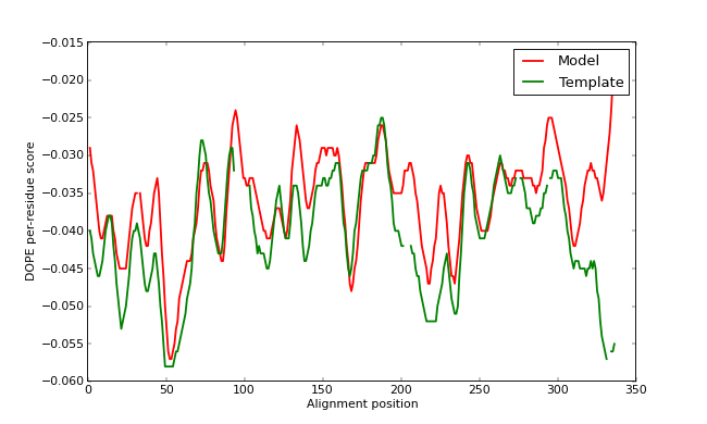
DOPE score profiles for the model and templates
This long loop interacts with region 220-250, which forms the other half of the active site. This latter part is well resolved in the template and probably correctly modeled in the target structure, but due to the unfavorable non-bonded interactions with the 90-100 region, it is also reported to be of high "energy" by DOPE. In general, a possible error indicated by DOPE may not necessarily be an actual error, especially if it highlights an active site or a protein-protein interface. However, in this case, the same active site loops have a better profile in the template structure, which strengthens the assessment that the model is probably incorrect in the active site region. This problem is addressed in the advanced modeling tutorial.