

Modeling with cryo-EM
Step 6: Fit models into cryo-EM maps
For this step of the tutorial, all input and output files can be found in the step6_fit directory of the file archive available on the index page.
Now that it has been demonstrated how to build a comparative model using only its sequence and a set of known crystal structures, how can cryo-EM data be added into this procedure? A map of the TvLDH structure is provided for this tutorial at 10Å resolution (TvLDH.10A.mrc). One solution that is explored in this step is to perform rigid fitting, using the Mod-EM method implemented in MODELLER (Topf et al., J. Struct. Biol. 149, 191-203, 2005). The script below carries out rigid translations and rotations of the protein in order to fit it into the map, in practice by maximizing the cross correlation between the map's density and a simulated density for the protein.
from modeller import *

log.verbose()
env = Environ()

struct='../step4_model/TvLDH.B99990001.pdb'
map='TvLDH.10A.mrc'
resolution=10.0
box_size=48
apix=1.88
x=-26.742; y=-9.5205; z=-10.375 #origin
steps=20

# Read in cryo-EM density map
den = Density(env, file=map, em_density_format='MRC',
              voxel_size=apix, resolution=resolution, em_map_size=box_size,
              density_type='GAUSS', px=x,py=y,pz=z)

# Fit the PDB file into the map by MC simulated annealing
den.grid_search(em_density_format='MRC', num_structures=1,
                em_pdb_name=struct, chains_num=[1],
                start_type='CENTER', number_of_steps=steps,
                angular_step_size=30., temperature=100.,
                best_docked_models=1, translate_type='RANDOM',
                em_fit_output_file='modem.log')
File: modem_mc.py
There are a variety of parameters for controlling the reading of cryo-EM maps and the grid_search method; see the MODELLER manual for full details. In this case, the fit is performed using a Monte Carlo optimization. The result of running the script is a new PDB file, TvLD_1_1.pdb, which contains the transformed coordinates of the protein to best fit it in the map. The log file contains details on the fit, such as the cross correlation. This is very good in the example outputs (0.9381). This combined with a visual inspection of the fit (see below) strongly suggests that the model is a good one - i.e. the chosen template is reasonable, MODELLER has correctly identified the fold of the target protein, and the alignment is probably largely correct. (Note that because generated PDB files may differ between computers, the exact value of the CCF may also differ.)
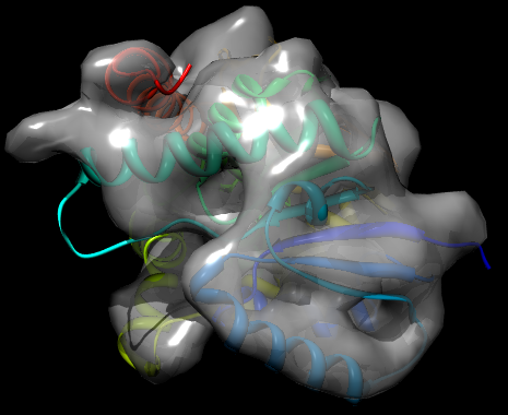
Fit of TvLDH structure into the EM map, rendered by Chimera and POV-Ray
While fitting a given model into a map can be computationally expensive, if the models are already fit into the map, the CCF can be calculated much more quickly. This is done in the script below (fitall.py) by first superposing each of the five generated models onto the fit conformation from the previous step, TvLD_1_1.pdb. The CCF is then calculated by adding the density-fit score into the MODELLER scoring function and then calling energy().
from __future__ import print_function
from modeller import *
from modeller.scripts import complete_pdb

log.verbose()
env = Environ()
env.libs.topology.read('${LIB}/top_heav.lib')
env.libs.parameters.read('${LIB}/par.lib')

# cryo-EM map details
map='TvLDH.10A.mrc'
resolution=10.0
box_size=48
apix=1.88
x=-26.742; y=-9.5205; z=-10.375 #origin

# Read in already-fitted PDB file and select all C-alpha atoms
m1 = Model(env, file='TvLD_1_1.pdb')
sel = Selection(m1).only_atom_types('CA')

scal = physical.Values(default=0., em_density=1.0)
results = []

# Loop over all five output PDB files
for i in range(1, 6):
    # Read in the output PDB file
    fname = '../step4_model/TvLDH.B9999%04d.pdb' % i
    m2 = complete_pdb(env, fname)

    # Make a 1:1 alignment of the already-fitted file and this model
    aln = Alignment(env)
    aln.append_model(m1, align_codes='fitted')
    aln.append_model(m2, align_codes='model')

    # Structural superposition using sel (all C-alpha positions)
    sel.superpose(m2, aln)

    # Read in cryo-EM map
    den = Density(env, file=map, em_density_format='MRC',
                  voxel_size=apix, resolution=resolution, em_map_size=box_size,
                  density_type='GAUSS', px=x,py=y,pz=z)

    # Add the EM density fit score (negative of CCF) to the MODELLER
    # scoring function for this model
    m2.env.edat.density = den

    # Calculate scoring function (energy) for all atoms in m2, with all
    # scoring function terms except the EM density fit score turned off
    # (scaled to zero)
    molpdf, terms = Selection(m2).energy(schedule_scale=scal)
    results.append((fname, -molpdf))

# Print all results
print("\n%-40s %12s" % ('Filename', 'CCF'))
print("\n".join(['%-40s %12.4f' % x for x in results]))
File: fitall.py
As can be seen from the resulting log file (shown below), all five of the generated models using this template yield good CCF scores. There is little variation in CCF between the five models. This is, however, not surprising - for good models generated from a good alignment, the differences are likely to be only in sidechain packing and some loop orientations, and a 10Å map probably does not have sufficient resolution to distinguish sidechains. (Note that because generated PDB files may differ between computers, the exact value of the CCFs may also differ.)
Filename                                          CCF
../step4_model/TvLDH.B99990001.pdb             0.9381
../step4_model/TvLDH.B99990002.pdb             0.9389
../step4_model/TvLDH.B99990003.pdb             0.9391
../step4_model/TvLDH.B99990004.pdb             0.9393
../step4_model/TvLDH.B99990005.pdb             0.9386
Excerpts of the file fitall.log
A map at 10Å resolution does suffice, however, to spot a poor alignment or choice of template. For example, in step 1 a number of potential templates were identified, any one of which could be used to build models of TvLDH. One such template is 2cmd:A, which was rejected due to its higher e-value and lower sequence identity. The 2cmd directory for this tutorial contains scripts to build, assess, and fit models of TvLDH using this template (run align2d.py, model-single.py and modem_mc.py in order). By inspection of the final output file modem_mc.log, it can be seen that the resulting model fits less well into the map - in the sample results, the CCF is lowered to 0.9057.