

Modeling with cryo-EM
Step 8: Flexible cryo-EM fitting with Flex-EM
For this step of the tutorial, all input and output files can be found in the step8_flexible directory of the file archive available on the index page.
The rigid fitting method explored earlier suffers from a number of disadvantages. Since it is applied only after the modeling procedure is complete, it can be used only as a filter or assessment method, and the information in the map is not fully utilized to guide the modeling or loop refinement itself. The conformation of the model structure may also differ from that of the template, due to loop distortions, movement of secondary structure elements, or errors introduced in the comparative modeling procedure itself (e.g. incorrect alignment). These problems can be overcome by using a flexible fitting method, whereby the protein structure is optimized simultaneously using the fit into the cryo-EM map and the regular scoring function incorporating stereochemistry and nonbonded interactions.
Full details on the so-called Flex-EM method can be found on its website and the accompanying publication, Topf et al., Structure 16, 295-307, 2008.
For this demonstration a model of 1ake:A generated by MODELLER using 1dvr:B as the template is refined using a 10Å cryo-EM map of 1ake:A. In a rigorous application, using several cycles of conjugate gradients and simulated annealing optimization, this reduced the RMSD of the model compared to the native structure from roughly 4.5Å to 2.2Å. This demonstration uses a less rigorous optimization than that employed for the Flex-EM publication, skipping the initial conjugate gradients optimization and performing only one annealing cycle, but will still take several hours to complete. Thus, it is best run overnight.
To actually run the simulation, first the Flex-EM Python files must be downloaded from the Flex-EM website. These are included in the file archive, with minor changes to MD.py to reduce the amount of optimization. Next, the control file flex-em.py must be modified (as below) to define the type of optimization, the input PDB file, and the cryo-EM map.
#  ============================================================================
#
#  a. Define the type of oprimization: conjugate gradients minimization (CG)
#     or molecular dynamics (MD)
#  b. Edit input parameters: density map parameters and probe structure
#
#  =======================  Maya Topf, 4 Dec 2007 =============================

from modeller import *
import shutil
import sys, os, os.path
import string
import math
from CG import opt_cg
from MD import opt_md

env = environ()

############### INPUT PARAMETERS ##################
optimization = 'MD'                     # type of optimization: CG / MD
rigid_filename = 'rigid.txt'            # rigid bodies file name
path = './'                             # directory path
code = '1ake'                           # 4 letter code of the structure
input_pdb_file = '1ake_init.pdb'        # input model for optimization
em_map_file = '1ake_10A.mrc'            # name of EM density map (mrc)
format='MRC'                            # map format: MRC or XPLOR
apix=1.0                                # voxel size: A/pixel
box_size=69                             # size of the density map (cubic)
resolution=10.0                         # resolution
x=-9.0; y=14.0; z=-8.0                  # origin of the map
num_of_runs = 1                         # number of runs
initial_dir = 1

############### RUN OPTIMIZATION ##################
#  CG
# ----
if optimization == 'CG':
    for i in range(initial_dir,initial_dir+num_of_runs):
        scratch = path + '/' + str(i) + '/'
        os.system("mkdir -p " + scratch)
        os.system("cp " + path + '/'+ input_pdb_file + " " + scratch)
        os.chdir(scratch)
        opt_cg(path, code, str(i), 55*i, em_map_file, input_pdb_file,
                format, apix, box_size, resolution, x, y, z, rigid_filename)

#  MD
# ----
elif optimization == 'MD':
    for i in range(initial_dir,initial_dir+num_of_runs):
        scratch = path + '/' + str(i) + '/'
#       input_pdb_file = 'final' + str(i) + '_cg.pdb'
#       os.chdir(scratch)
        opt_md(path, code, str(i), 10*i, em_map_file, input_pdb_file,
                format, apix, box_size, resolution, x, y, z, rigid_filename)
File: flex-em.py
In order to reduce the conformational space that must be searched during this procedure, groups of atoms (for example, secondary structure elements) can be defined and moved as rigid bodies. This is done by creating a file rigid.txt.
helix
13   24 nr
31   41 nr
44   54 nr
61   73 nr
76   79 nr
90   99 nr
113   122 nr
161   185 nr
202   212 nr
beta
2   6   28   30   81   84   105   110   193   197 nr
123   126   132   134   153   154 nr
File: rigid.txt
The script can be run in the usual way; on completion it generates a file final1_mdcg.pdb containing a new PDB structure that has been refined by flexible fitting into the map. By visual inspection of the initial structure (white) and the fitted structure (purple) below, it can clearly be seen that several secondary structure elements have moved towards the density. The file archive also contains a script superpose.py that can be used to superpose the final and fitted structures on the known (native) structure of 1ake:A. This shows a reduction in the RMSD from approximately 4.5 to 3.5Å.
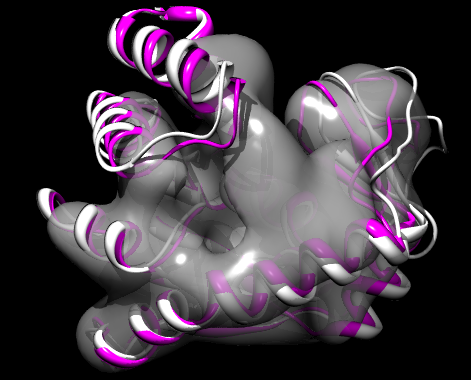
Fit of 1ake:A initial structure (white) and Flex-EM refined structure (purple) into EM map, rendered with Chimera and POV-Ray